by R. Grothmann
Let me demonstrate the use of numerical analysis with Euler for real world problems.
The problem we wish to investigate is shooting a canon ball with speed v and angle a. This can, of course, be computed exactly. But first we restrict ourselves to numerical solutions.
We fix the speed v=10 m/s and approximate the gravitation with g=10 m/s^2.
>v=10; g=10;
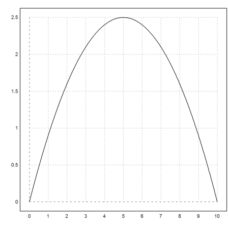
Now we plot a specific ballistic curve for a canon ball fired at 45° with the well known formulas for the curve neglecting friction.
Time runs from 0 s to 2 s.
>t=0:0.1:2;
The movement in x-direction (height) is
![]()
The movement in y-direction is
![]()
>function x(t,a) := cos(a)*v*t; ...
 function y(t,a) := sin(a)*v*t-g*t^2/2; ...
 plot2d(x(t,45°),y(t,45°)):
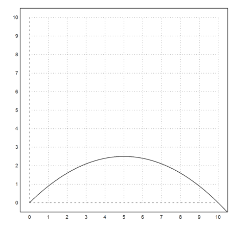
We notice that we are not interested in the negative y-values and clip the plot to the positive quadrant.
>plot2d(x(t,45°),y(t,45°),a=0,b=10,c=0,d=10):
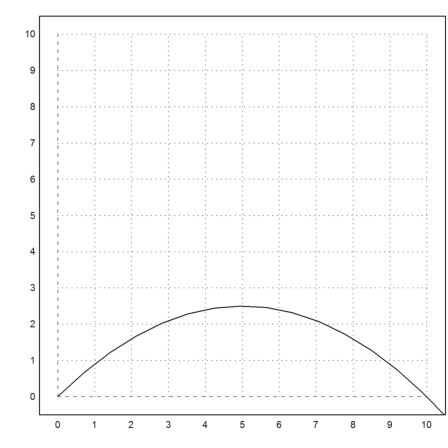
We now compute the time, at which the ball has its highest altitude. We use the function fmax(), which computes the maximum of a function or expression in a given range.
>tmax=fmax("y(x,45°)",0,2)
0.707106772995
How high is the maximal height?
>y(tmax,45°)
2.5
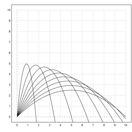
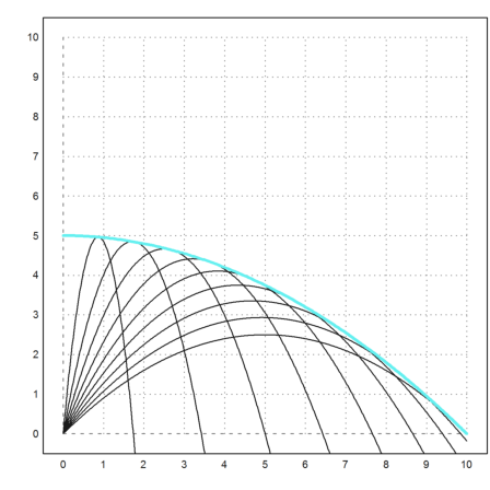
We wish to compare several angles. Thus we generate a vector of angles from 5° to 85° and generate all curves for all these angles simultaneously.
To do so, we need the angle a as a column vector and the time t as a row vector. Combining both yields a matrix, with a curve in each row for each angle.
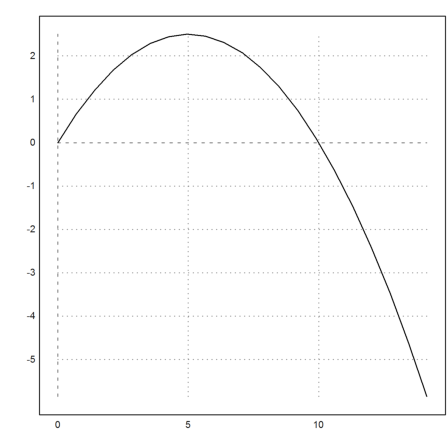
>a=(5:5:85)°; a=a'; ...
 plot2d(x(t,a),y(t,a),a=0,b=10,c=0,d=10):
Lets us now compute the distance from the origin to the contact of the ball with the ground. We use the simplest of methods, the bisection method.
We seek the zero of y(x,a). The additional parameter a (after the semicolon) is passed from bisect to y.
Note: Our function will only work for scalar a, not for vectors a, if we do not map.
>function map distance (a) := x(bisect("y",0,2;a),a);
What happens, if we take 50°?
>distance(50°)
9.84807753012
We get about 9.85m.
Let us plot the impact distance with varying angles.
>a=(1:1:89)°;
To compute the impact function for all angles, we apply "distance" to the vector a. The function is mapped to all elements of a.
>plot2d(deg(a),map("distance",a)):
We can also compute the optimal angle and its distance.
>amax=fmax("distance",1°,89°); deg(amax), distance(amax),
44.9999773572
9.99999999999
Of course, it is easy to invert the function x, i.e., compute the time t for the value x. We would not need to have done that numerically.
So we write a function that computes the height of the ball at distance x, if the angle is a.
>function height (x,a) := y(x/(cos(a)*v),a)
Test this with 45° from 0 to 10.
>plot2d("height";45°,a=0,b=10):
We now want to get as high as possible in 5m distance. Again, we use fmax, but the argument x is now the second parameter to the function height, the angle.
>degprint(fmax("height(5,x)",1°,89°))
63°26'5.82''
We need the angle argument as first argument for the next function.
>function height1(a,x) := height(x,a)
Now, we make a function that computes the angles that yields the maximal heights for given distances. Since fmax calls height to maximize the angle, we call height1(x,xx).
>function heighestangle (xx) := fmax("height1",1°,89°;xx)
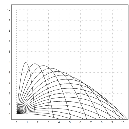
Compute various maximal heights and plot them together with some shots.
>x=0.2:0.05:10; y=map("heighestangle",x); ...
 plot2d(x,height(x,y),color=red,thickness=2); ...
 a=(5°:5°:85°)'; plot2d(x(t,a),y(t,a),add=1):
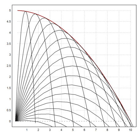
Is the curve of maximal heights a parabola?
Yes it is. To demonstrate, we compute the interpolation polynomial of second degree through the know values at -10, 0 and 10.
>d=interp([-10,0,10],[0,5,0]);
Then we plot the polynomial over the current view in color 13. Indeed, we get the same curve.
>plot2d("interpval([-10,0,10],d,x)",add=1,color=10,thickness=3):
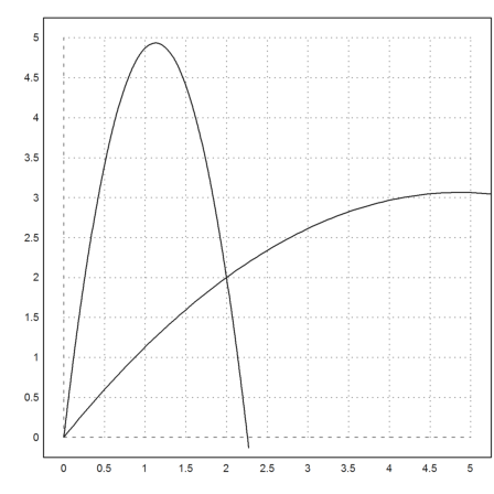
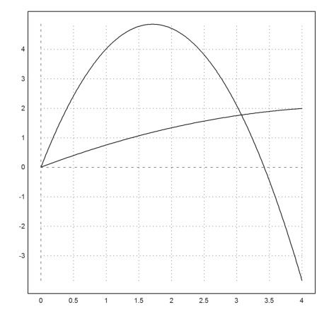
Next, we ask how to reach the point x=2, y=2. There seem to be two solutions. We get both by searching the angle below and the angle above the one with maximal height.
>a=heighestangle(2); degprint(a)
78°41'24.24''
>height(2,a)
4.8
>a1=bisect("height(2,x)-2",0,a); degprint(a1)
51°31'33.49''
>a2=bisect("height(2,x)-2",a,pi/2); degprint(a2)
83°28'26.51''
Let's plot both solutions to one plot.
>t=0:0.01:2; ...
 plot2d(x(t,a1),y(t,a1),a=0,b=5,c=0,d=5); ...
 plot2d(x(t,a2),y(t,a2),add=1):
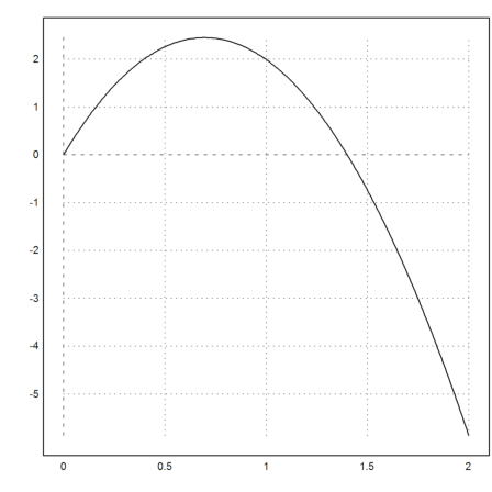
Assume we shoot a ball in 80° and another one in 40°. Can we hit the first with the second in the air?
We plot the two paths.
>plot2d("height(x,80°)",a=0,b=4); plot2d("height(x,40°)",add=1):
Now we compute the point, where both paths meet and compute the time difference.
>xd=bisect("height(x,80°)-height(x,40°)",0.001,5)
3.07201661702
>xd/(v*cos(80°))-xd/(v*cos(40°))
1.3680805733
Now we introduce friction. We assume the friction force is proportional to c*v, where v is the speed.
We need to solve a differential equation, using the "runge" function. The state x of the ball at any time t is 4-dimensional and contains two point coordinates and two speed coordinates. We need a function to compute x'=f(t,x).
We set x=[sx,sy,sx',sy'].
>function f(t,x,c=0.005) ...
 global g;
 v=sqrt(x[3]*x[3]+x[4]*x[4]); rho=c*v;
 return [x[3],x[4],-rho*x[3],-g-rho*x[4]]
 endfunction
We need to pass a vector of times t, where x will be computed. "runge" returns a matrix s, with one value for s in each column. We may plot the path of the ball from the first two rows of s.
>t=0:0.01:2; s=ode("f",t,[0,0,cos(45°)*v,sin(45°)*v]); ...
 plot2d(s[1],s[2],a=0,b=10,c=0,d=10);
As you see, we get a little shorter.
>plot2d(x(t,45°),y(t,45°),add=1,color=blue):
Now we look at the speed over a larger time. The speed will tend to some value, where friction is equal to gravity.
>t=0:0.01:20; s=ode("f",t,[0,0,cos(45°)*v,sin(45°)*v]);
>plot2d(t,sqrt(s[3]^2+s[4]^2)):
We wish to compute the angle of maximal width for this problem. It will no longer be exactly 45°.
First we define a function returning the height at time t.
>function height (t,a) ...
 global v;
 s=runge("f",[0,t],[0,0,cos(a)*v,sin(a)*v],20);
 return s[2,2];
 endfunction
>plot2d("height";45°,a=0,b=2):
Then we seek the time when the height is 0 for any angle a, and return the width at that time.
>function width (a) ...
 t=bisect("height",0.001,2;a);
 global v;
 s=runge("f",[0,t],[0,0,cos(a)*v,sin(a)*v],20);
 return s[1,2];
 endfunction
>width(45°)
9.62578470286
Now we maximize the width over the angles.
We find that the optimal angle is slightly less than 45°.
>amax=fmax("width",30°,60°); degprint(amax)
44°42'25.31''
Now we compute ballistic shots with Maxima, with and without air resistance.
First the x-coordinate of the shot path (neglecting friction).
>function sx(v,t,a) &= v*t*cos(a)
cos(a) t v
For the y-coordinate we subtract the influence of gravity.
>function sy(v,t,a) &= v*t*sin(a)-g*t^2/2
                                          2
                                       g t
                          sin(a) t v - ----
                                        2
Let us plot a sample shot.
>v=10; g=10; a=%pi/4; plot2d("sx(v,x,a)","sy(v,x,a)", ...
 a=0,b=10,c=0,d=10,xmin=0,xmax=2):
Now we solve for the time, when the ball hits the ground.
>&solve(sy(v,t,a)=0,t), function wa(v,a) &= at(sx(v,t,a),%[1])
                            2 sin(a) v
                       [t = ----------, t = 0]
                                g


                                           2
                          2 cos(a) sin(a) v
                          ------------------
                                  g
Let us plot the width with varying angles.
>plot2d("wa(v,rad(x))",0,90):
We can compute the angle of maximum distance numerically in Euler.
>deg(fmax("wa(v,x)",0,90°))
44.9999996766
The same in Maxima using calculus.
>&solve(diff(wa(v,a),a)=0,a)
[sin(a) = - cos(a), sin(a) = cos(a)]
We need to help Maxima.
>&solve(trigreduce(diff(wa(v,a),a))=0,a)
                                    pi
                               [a = --]
                                    4
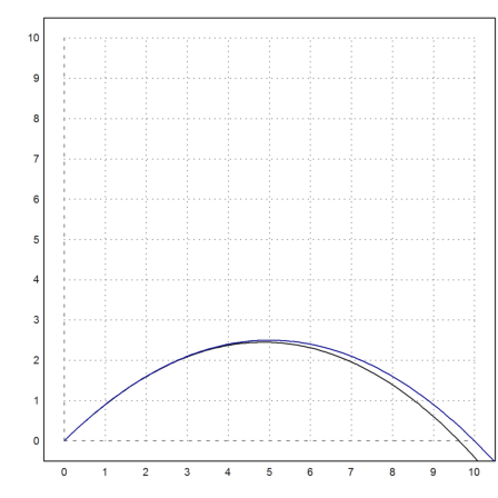
Let us compute the height of a ball at distance x.
>&solve(sx(v,t,a)=x,t), function hx(x,v,a) &= ratsimp(at(sy(v,t,a),%))
                                    x
                            [t = --------]
                                 cos(a) v


                                      2        2
                     2 cos(a) sin(a) v  x - g x
                     ---------------------------
                                 2     2
                            2 cos (a) v
Plot a shot at angle 45°.
>plot2d("hx(x,v,45°)",a=0,b=10,c=0,d=10):
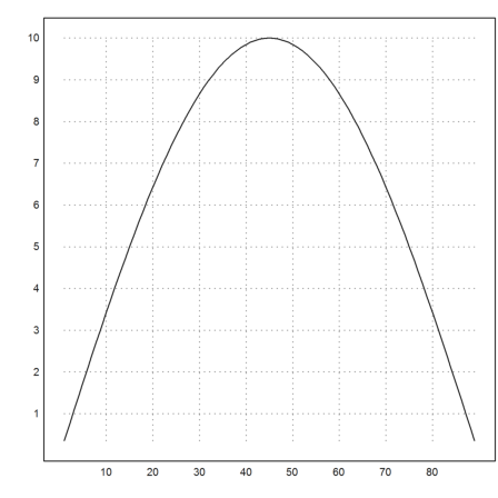
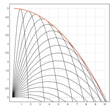
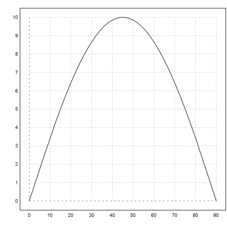
Now we use the Euler matrix language to plot shots for angles from 45° to 90°.
>x:=0:0.01:10; y:=hx(x,v,(45°:5°:90°)'); ...
 plot2d(x,y,a=0,b=10,c=0,d=10):
We wish to compute the resultant. In this case, it the maximal height one can reach at distance x.
>&trigsimp(diff(hx(x,v,a),a)), &solve(%=0,a)
                              2               2
                      cos(a) v  x - sin(a) g x
                      -------------------------
                                3     2
                             cos (a) v


                                           2
                                   cos(a) v
                         [sin(a) = ---------]
                                      g x
This is not quite complete, but we can use it nevertheless.
>function par(x,v) &= ratexpand(at(hx(x,v,a),a=expand(atan(v^2/(g*x)))))
                               2       2
                              v     g x
                              --- - ----
                              2 g      2
                                    2 v
We add this parabola to the plot above.
>plot2d("par(x,v)",add=1,color=13,thickness=3):
This does also answer the question, how far we can get if we aim from some level b different from 0.
E.g., assume we are b meters above ground and throw a stone with speed v at an optimal angle, at gravity g. The distance is then our resolvent at y=-b.
>&solve(par(x,v)=-b,x)[2]
                                    2
                            v sqrt(v  + 2 b g)
                        x = ------------------
                                    g
To find the optimal angle for such a throw, we need tu use numerical methods. First we find the distance, we can reach, if we use an angle a.
>&solve(sy(v,t,a)=-b,t), function wa(a,v) &= at(sx(v,t,a),%[2])
                                2     2
             sin(a) v - sqrt(sin (a) v  + 2 b g)
        [t = -----------------------------------,
                              g
                                          2     2
                                  sqrt(sin (a) v  + 2 b g) + sin(a) v
                              t = -----------------------------------]
                                                   g


                              2     2
            cos(a) v (sqrt(sin (a) v  + 2 b g) + sin(a) v)
            ----------------------------------------------
                                  g
We use the Euler fmax function to find the angle for the maximal distance at height 5, with v=10, g=10 as above.
>v:=10; g:=10; b:=5; deg(fmax("wa(x,v)",0,90°))
35.2643895179
Let us try to add some air resistance. However, we can only solve that equation exactly, if we assume the air resistance is quadratic with the speed and that we simply drop the body.
We set up a differential equation for the speed at time x.
>eq1 &= 'diff(v(x),x) = -g+k*v(x)^2
                       d              2
                       -- (v(x)) = k v (x) - g
                       dx
This can be solved.
>&assume(g>0); &assume(k>0); sol &= ode2(eq1,v(x),x)
                    k v(x) - sqrt(g) sqrt(k)
                log(------------------------)
                    k v(x) + sqrt(g) sqrt(k)
                ----------------------------- = x + %c
                      2 sqrt(g) sqrt(k)
The solution is implicit. We need to solve for v(x) first, and assign the solution to sol(x).
>function sol(x) &= ratsimp(rhs(solve(sol,v(x))[1]))
                       2 sqrt(g) sqrt(k) x + 2 %c sqrt(g) sqrt(k)
     sqrt(g) sqrt(k) (E                                           + 1)
   - -----------------------------------------------------------------
                2 sqrt(g) sqrt(k) x + 2 %c sqrt(g) sqrt(k)
             k E                                           - k
Next we determine the constant %c, so that the speed at x=0 is 0.
>constants &= solve(sol(0)=0,%c)
                      log(- I)               log(I)
             [%c = ---------------, %c = ---------------]
                   sqrt(g) sqrt(k)       sqrt(g) sqrt(k)
Substitute the solution into sol(x) and fix sol(x).
>function solution(x) &= at(sol(x),constants[2])
                                     2 sqrt(g) sqrt(k) x
               sqrt(g) sqrt(k) (1 - E                   )
             - ------------------------------------------
                           2 sqrt(g) sqrt(k) x
                      - k E                    - k
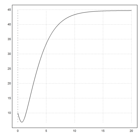
Next we plot the speed versus the time. As expected, we get a limit speed.
>k:=0.01; plot2d("solution(x)",0,40):
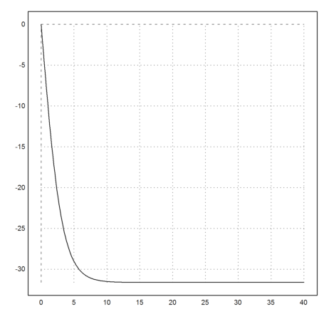
We can find this limit exactly with Maxima.
>&limit(solution(x),x,inf)|k=1/100|g=10, %()
                                   3/2
                               - 10

-31.6227766017
Now we integrate the speed and find the drop length at time a.
>&assume(x>0); function h(x) &= integrate(solution(t),t,0,x)
                2 sqrt(g) sqrt(k) x
           log(E                    + 1)   sqrt(g) x   log(2)
         - ----------------------------- + --------- + ------
                         k                  sqrt(k)      k
If we plot this, it looks like a parabola.
>plot2d("h(x)",0,5):
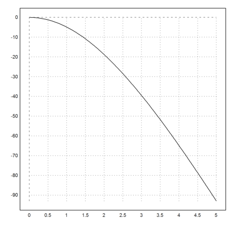
With k=0, this converges to a parabola. We need to compute the limit using Taylor a series expansion.
>&tlimit(h(x),k,0)
                                     2
                                  g x
                                - ----
                                   2